Tracy–Widom distribution

The Tracy–Widom distribution is a probability distribution from random matrix theory introduced by Craig Tracy and Harold Widom (1993, 1994). It is the distribution of the normalized largest eigenvalue of a random Hermitian matrix. The distribution is defined as a Fredholm determinant.

In practical terms, Tracy–Widom is the crossover function between the two phases of weakly versus strongly coupled components in a system. It also appears in the distribution of the length of the longest increasing subsequence of random permutations, as large-scale statistics in the Kardar-Parisi-Zhang equation, in current fluctuations of the asymmetric simple exclusion process (ASEP) with step initial condition, and in simplified mathematical models of the behavior of the longest common subsequence problem on random inputs. See Takeuchi & Sano (2010) and Takeuchi et al. (2011) for experimental testing (and verifying) that the interface fluctuations of a growing droplet (or substrate) are described by the TW distribution ${\displaystyle F_{2}}$ (or ${\displaystyle F_{1}}$) as predicted by Prähofer & Spohn (2000).

The distribution ${\displaystyle F_{1}}$ is of particular interest in multivariate statistics. For a discussion of the universality of ${\displaystyle F_{\beta }}$, ${\displaystyle \beta =1,2,4}$, see Deift (2007). For an application of ${\displaystyle F_{1}}$ to inferring population structure from genetic data see Patterson, Price & Reich (2006). In 2017 it was proved that the distribution F is not infinitely divisible.

Definition as a law of large numbers

Let ${\displaystyle F_{\beta }}$ denote the cumulative distribution function of the Tracy–Widom distribution with given ${\displaystyle \beta }$. It can be defined as a law of large numbers, similar to the central limit theorem.

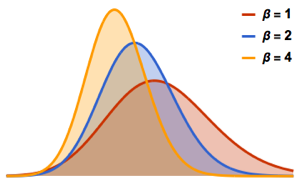
There are typically three Tracy–Widom distributions, ${\displaystyle F_{\beta }}$, with ${\displaystyle \beta \in \{1,2,4\}}$. They correspond to the three gaussian ensembles: orthogonal (${\displaystyle \beta =1}$), unitary (${\displaystyle \beta =2}$), and symplectic (${\displaystyle \beta =4}$).

In general, consider a gaussian ensemble with beta value ${\displaystyle \beta }$, with its diagonal entries having variance 1, and off-diagonal entries having variance ${\displaystyle \sigma ^{2}}$, and let ${\displaystyle F_{N,\beta }(s)}$ be probability that an ${\displaystyle N\times N}$ matrix sampled from the ensemble have maximal eigenvalue ${\displaystyle \leq s}$, then define$${\displaystyle F_{\beta }(x)=\lim _{N\to \infty }F_{N,\beta }(\sigma (2N^{1/2} N^{-1/6}x))=\lim _{N\to \infty }Pr(N^{1/6}(\lambda _{max}/\sigma -2N^{1/2})\leq x)}$$where ${\displaystyle \lambda _{\max }}$ denotes the largest eigenvalue of the random matrix. The shift by ${\displaystyle 2\sigma N^{1/2}}$ centers the distribution, since at the limit, the eigenvalue distribution converges to the semicircular distribution with radius ${\displaystyle 2\sigma N^{1/2}}$. The multiplication by ${\displaystyle N^{1/6}}$ is used because the standard deviation of the distribution scales as ${\displaystyle N^{-1/6}}$ (first derived in ).

For example:

${\displaystyle F_{2}(x)=\lim _{N\to \infty }\operatorname {Prob} \left((\lambda _{\max }-{\sqrt {4N}})N^{1/6}\leq x\right),}$

where the matrix is sampled from the gaussian unitary ensemble with off-diagonal variance ${\displaystyle 1}$.

The definition of the Tracy–Widom distributions ${\displaystyle F_{\beta }}$ may be extended to all ${\displaystyle \beta >0}$ (Slide 56 in Edelman (2003), Ramírez, Rider & Virág (2006)).

One may naturally ask for the limit distribution of second-largest eigenvalues, third-largest eigenvalues, etc. They are known.

Functional forms

Fredholm determinant

${\displaystyle F_{2}}$ can be given as the Fredholm determinant

${\displaystyle F_{2}(s)=\det(I-A_{s})=1 \sum _{n=1}^{\infty }{\frac {(-1)^{n}}{n!}}\int _{(s,\infty )^{n}}\det _{i,j=1,...,n}[A_{s}(x_{i},x_{j})]dx_{1}\cdots dx_{n}}$

of the kernel ${\displaystyle A_{s}}$ ("Airy kernel") on square integrable functions on the half line ${\displaystyle (s,\infty )}$, given in terms of Airy functions Ai by

${\displaystyle A_{s}(x,y)={\begin{cases}{\frac {\mathrm {Ai} (x)\mathrm {Ai} '(y)-\mathrm {Ai} '(x)\mathrm {Ai} (y)}{x-y}}\quad {\text{if }}x\neq y\\Ai'(x)^{2}-x(Ai(x))^{2}\quad {\text{if }}x=y\end{cases}}}$

Painlevé transcendents

${\displaystyle F_{2}}$ can also be given as an integral

${\displaystyle F_{2}(s)=\exp \left(-\int _{s}^{\infty }(x-s)q^{2}(x)\,dx\right)}$

in terms of a solution of a Painlevé equation of type II

${\displaystyle q^{\prime \prime }(s)=sq(s) 2q(s)^{3}\,}$

with boundary condition ${\textstyle \displaystyle q(s)\sim {\textrm {Ai}}(s),s\to \infty .}$ This function ${\displaystyle q}$ is a Painlevé transcendent.

Other distributions are also expressible in terms of the same ${\displaystyle q}$:

${\displaystyle {\begin{aligned}F_{1}(s)&=\exp \left(-{\frac {1}{2}}\int _{s}^{\infty }q(x)\,dx\right)\,\left(F_{2}(s)\right)^{1/2}\\F_{4}(s/{\sqrt {2}})&=\cosh \left({\frac {1}{2}}\int _{s}^{\infty }q(x)\,dx\right)\,\left(F_{2}(s)\right)^{1/2}.\end{aligned}}}$

Functional equations

Define $${\displaystyle {\begin{aligned}F(x)&=\exp \left(-{\frac {1}{2}}\int _{x}^{\infty }(y-x)q(y)^{2}\,dy\right)\\E(x)&=\exp \left(-{\frac {1}{2}}\int _{x}^{\infty }q(y)\,dy\right)\end{aligned}}}$$then$${\displaystyle F_{1}(x)=E(x)F(x),\quad F_{2}(x)=F(x)^{2},\quad \quad F_{4}\left({\frac {x}{\sqrt {2}}}\right)={\frac {1}{2}}\left(E(x) {\frac {1}{E(x)}}\right)F(x)}$$

Occurrences

Other than in random matrix theory, the Tracy–Widom distributions occur in many other probability problems.

Let ${\displaystyle l_{n}}$ be the length of the longest increasing subsequence in a random permutation sampled uniformly from ${\displaystyle S_{n}}$, the permutation group on n elements. Then the cumulative distribution function of ${\displaystyle {\frac {l_{n}-2N^{1/2}}{N^{1/6}}}}$ converges to ${\displaystyle F_{2}}$.

Third-order phase transition

The Tracy–Widom distribution exhibits a third-order phase transition in the large deviation behavior of the largest eigenvalue of a random matrix. This transition occurs at the edge of the Wigner semicircle distribution, where the probability density of the largest eigenvalue follows distinct scaling laws depending on whether it deviates to the left or right of the edge.

Let ${\displaystyle \Phi (w)}$ denote the rate function governing the large deviations of the largest eigenvalue ${\displaystyle \lambda _{\max }}$. For a Gaussian unitary ensemble, the probability density function of ${\displaystyle \lambda _{\max }}$ satisfies, for large ${\displaystyle N}$,

${\displaystyle P(\lambda _{\max }=w)\approx \exp \left(-\beta N^{p}\Phi (w)\right),}$

where ${\displaystyle p=2}$ for deviations to the left of the spectral edge and ${\displaystyle p=1}$ for deviations to the right. When the small-deviation parts of the probability density are included, we have$${\displaystyle P\left(\lambda _{\max }=w,N\right)\approx {\begin{cases}\exp \left[-\beta N^{2}\Phi _{-}(w)\right]&,w<{\sqrt {2}}\&|w-{\sqrt {2}}|\sim {\mathcal {O}}(1)\\{\sqrt {2}}N^{\frac {2}{3}}{\mathcal {F}}_{\beta }^{\prime }\left({\sqrt {2}}N^{\frac {2}{3}}(w-{\sqrt {2}})\right)&,\\\exp \left[-\beta N\Phi _{ }(w)\right]&,w>{\sqrt {2}}\&|w-{\sqrt {2}}|\sim {\mathcal {O}}\left(N^{-{\frac {2}{3}}}\right)\end{cases}}}$$

The rate function ${\displaystyle \Phi (w)}$ is given by separate expressions for ${\displaystyle w<{\sqrt {2}}}$ and ${\displaystyle w>{\sqrt {2}}}$. $${\displaystyle {\begin{aligned}\Phi _{-}(w)=&{\frac {1}{108}}\left[36w^{2}-w^{4}-\left(15w w^{3}\right){\sqrt {w^{2} 6}}\right.\\&\left. 27\left(\ln 18-2\ln \left(w {\sqrt {w^{2} 6}}\right)\right)\right],w<{\sqrt {2}}.\end{aligned}}}$$

$${\displaystyle \Phi _{ }(w)={\frac {1}{2}}w{\sqrt {w^{2}-2}} \ln \left[{\frac {w-{\sqrt {w^{2}-2}}}{\sqrt {2}}}\right]}$$

Near the critical point ${\displaystyle w={\sqrt {2}}}$, the leading order behavior is

${\displaystyle \Phi _{-}(w)\sim {\frac {1}{6{\sqrt {2}}}}({\sqrt {2}}-w)^{3},\quad w\to {\sqrt {2}}^{-}.}$

${\displaystyle \Phi _{ }(w)\sim {\frac {2^{7/4}}{3}}(w-{\sqrt {2}})^{3/2},\quad w\to {\sqrt {2}}^{ }.}$

The third derivative of ${\displaystyle \Phi (w)}$ is discontinuous at ${\displaystyle w={\sqrt {2}}}$, which classifies this as a third-order phase transition. This type of transition is analogous to the Gross-Witten-Wadia phase transition in lattice gauge theory and the Douglas-Kazakov phase transition in two-dimensional quantum chromodynamics. The discontinuity in the third derivative of the free energy marks a fundamental change in the behavior of the system, where fluctuations transition between different scaling regimes.

This third-order transition has also been observed in problems related to the maximal height of non-intersecting Brownian excursions, conductance fluctuations in mesoscopic systems, and entanglement entropy in random pure states.

To interpret this as a third-order transition in statistical mechanics, define the (generalized) free energy density of the system as$${\displaystyle {\mathcal {F}}(w)=-{\frac {1}{N^{2}}}\ln P\left(\lambda _{\max }=w,N\right)}$$then at the ${\displaystyle N\to \infty }$ limit, ${\displaystyle {\mathcal {F}}(w)={\begin{cases}\Phi _{-}(w)&w<{\sqrt {2}}\\0&w>{\sqrt {2}}\end{cases}}}$ has continuous first and second derivatives at the critical point ${\displaystyle w={\sqrt {2}}}$, but a discontinuous third derivative.

The ${\displaystyle -\ln P\propto N^{2}}$ lower end can be interpreted as the strongly interacting regime, where ${\displaystyle N}$ objects are interacting strongly pairwise, so the total energy is proportional to ${\displaystyle N^{2}}$. The ${\displaystyle -\ln P\propto N}$ upper end can be interpreted as the weakly interacting regime, where the objects are basically not interacting, so the total energy is proportional to ${\displaystyle N}$. The Tracy–Widom distribution phase transition then occurs at the point as the system switches from strongly to weakly interacting.

Coulomb gas model

This can be visualized in the Coulomb gas model by considering a gas of electric charges in a ${\displaystyle V(x)={\frac {1}{2}}x^{2}}$ potential well. The distribution of the charges is the same as the distribution of the matrix eigenvalues. This gives the Wigner semi-circle law. To find the distribution of the largest eigenvalue, we take a wall and push against the Coulomb gas. If the wall is above ${\displaystyle {\sqrt {2}}}$, then most of the gas remains unaffected, and we are in the weak interaction regime. If the wall is below ${\displaystyle {\sqrt {2}}}$, then the entire bulk of the Coulomb gas is affected, and we are in the strong interaction regime.

The minimal Coulomb gas distribution is explicitly solvable as$${\displaystyle \rho _{w}^{*}(\lambda )={\begin{cases}{\frac {1}{\pi }}{\sqrt {2-\lambda ^{2}}},\quad {\text{ with }}\quad -{\sqrt {2}}\leq \lambda \leq {\sqrt {2}}&{\text{ for }}w>{\sqrt {2}}\\{\frac {\sqrt {\lambda L(w)}}{2\pi {\sqrt {w-\lambda }}}}[w L(w)-2\lambda ]\quad {\text{ with }}\quad -L(w)\leq \lambda \leq w&{\text{ for }}w<{\sqrt {2}}\end{cases}}}$$where ${\displaystyle w}$ is the position of the wall, and ${\displaystyle L(w)={\frac {2{\sqrt {w^{2} 6}}-w}{3}}}$.

Asymptotics

Probability density function

Let ${\displaystyle f_{\beta }(x)=F_{\beta }'(x)}$ be the probability density function for the distribution, then$${\displaystyle f_{\beta }(x)\sim {\begin{cases}e^{-{\frac {\beta }{24}}|x|^{3}},\quad x\to -\infty \\e^{-{\frac {2\beta }{3}}|x|^{3/2}},\quad x\to \infty \end{cases}}}$$In particular, we see that it is severely skewed to the right: it is much more likely for ${\displaystyle \lambda _{max}}$ to be much larger than ${\displaystyle 2\sigma {\sqrt {N}}}$ than to be much smaller. This could be intuited by seeing that the limit distribution is the semicircle law, so there is "repulsion" from the bulk of the distribution, forcing ${\displaystyle \lambda _{max}}$ to be not much smaller than ${\displaystyle 2\sigma {\sqrt {N}}}$.

At the ${\displaystyle x\to -\infty }$ limit, a more precise expression is (equation 49 )$${\displaystyle f_{\beta }(x)\sim \tau _{\beta }|x|^{(\beta ^{2} 4-6\beta )/16\beta }\exp \left[-\beta {\frac {|x|^{3}}{24}} {\sqrt {2}}{\frac {\beta -2}{6}}|x|^{3/2}\right]}$$for some positive number ${\displaystyle \tau _{\beta }}$ that depends on ${\displaystyle \beta }$.

Cumulative distribution function

At the ${\displaystyle x\to \infty }$ limit,$${\displaystyle {\begin{aligned}F(x)&=1-{\frac {e^{-{\frac {4}{3}}x^{3/2}}}{32\pi x^{3/2}}}{\biggl (}1-{\frac {35}{24x^{3/2}}} {\cal {O}}(x^{-3}){\biggr )},\\E(x)&=1-{\frac {e^{-{\frac {2}{3}}x^{3/2}}}{4{\sqrt {\pi }}x^{3/2}}}{\biggl (}1-{\frac {41}{48x^{3/2}}} {\cal {O}}(x^{-3}){\biggr )}\end{aligned}}}$$and at the ${\displaystyle x\to -\infty }$ limit,$${\displaystyle {\begin{aligned}F(x)&=2^{1/48}e^{{\frac {1}{2}}\zeta ^{\prime }(-1)}{\frac {e^{-{\frac {1}{24}}|x|^{3}}}{|x|^{1/16}}}\left(1 {\frac {3}{2^{7}|x|^{3}}} O(|x|^{-6})\right)\\E(x)&={\frac {1}{2^{1/4}}}e^{-{\frac {1}{3{\sqrt {2}}}}|x|^{3/2}}{\Biggl (}1-{\frac {1}{24{\sqrt {2}}|x|^{3/2}}} {\cal {O}}(|x|^{-3}){\Biggr )}.\end{aligned}}}$$where ${\displaystyle \zeta }$ is the Riemann zeta function, and ${\displaystyle \zeta '(-1)=-0.1654211437}$.

This allows derivation of ${\displaystyle x\to \pm \infty }$ behavior of ${\displaystyle F_{\beta }}$. For example,$${\displaystyle {\begin{aligned}1-F_{2}(x)&={\frac {1}{32\pi x^{3/2}}}e^{-4x^{3/2}/3}(1 O(x^{-3/2})),\\F_{2}(-x)&={\frac {2^{1/24}e^{\zeta ^{\prime }(-1)}}{x^{1/8}}}e^{-x^{3}/12}{\biggl (}1 {\frac {3}{2^{6}x^{3}}} O(x^{-6}){\biggr )}.\end{aligned}}}$$

Painlevé transcendent

The Painlevé transcendent has asymptotic expansion at ${\displaystyle x\to -\infty }$ (equation 4.1 of )$${\displaystyle q(x)={\sqrt {-{\frac {x}{2}}}}\left(1 {\frac {1}{8}}x^{-3}-{\frac {73}{128}}x^{-6} {\frac {10657}{1024}}x^{-9} O(x^{-12})\right)}$$This is necessary for numerical computations, as the ${\displaystyle q\sim {\sqrt {-x/2}}}$ solution is unstable: any deviation from it tends to drop it to the ${\displaystyle q\sim -{\sqrt {-x/2}}}$ branch instead.

Numerics

Numerical techniques for obtaining numerical solutions to the Painlevé equations of the types II and V, and numerically evaluating eigenvalue distributions of random matrices in the beta-ensembles were first presented by Edelman & Persson (2005) using MATLAB. These approximation techniques were further analytically justified in Bejan (2005) and used to provide numerical evaluation of Painlevé II and Tracy–Widom distributions (for ${\displaystyle \beta =1,2,4}$) in S-PLUS. These distributions have been tabulated in Bejan (2005) to four significant digits for values of the argument in increments of 0.01; a statistical table for p-values was also given in this work. Bornemann (2010) gave accurate and fast algorithms for the numerical evaluation of ${\displaystyle F_{\beta }}$ and the density functions ${\displaystyle f_{\beta }(s)=dF_{\beta }/ds}$ for ${\displaystyle \beta =1,2,4}$. These algorithms can be used to compute numerically the mean, variance, skewness and excess kurtosis of the distributions ${\displaystyle F_{\beta }}$.

Functions for working with the Tracy–Widom laws are also presented in the R package 'RMTstat' by Johnstone et al. (2009) and MATLAB package 'RMLab' by Dieng (2006).

For a simple approximation based on a shifted gamma distribution see Chiani (2014).

Shen & Serkh (2022) developed a spectral algorithm for the eigendecomposition of the integral operator ${\displaystyle A_{s}}$, which can be used to rapidly evaluate Tracy–Widom distributions, or, more generally, the distributions of the ${\displaystyle k}$th largest level at the soft edge scaling limit of Gaussian ensembles, to machine accuracy.

Tracy-Widom and KPZ universality

The Tracy-Widom distribution appears as a limit distribution in the universality class of the KPZ equation. For example it appears under ${\displaystyle t^{1/3}}$ scaling of the one-dimensional KPZ equation with fixed time.

See also

• Wigner semicircle distribution
• Marchenko–Pastur distribution

Footnotes

References

• Baik, J.; Deift, P.; Johansson, K. (1999), "On the distribution of the length of the longest increasing subsequence of random permutations", Journal of the American Mathematical Society, 12 (4): 1119–1178, arXiv:math/9810105, doi:10.1090/S0894-0347-99-00307-0, JSTOR 2646100, MR 1682248.
• Bornemann, F. (2010), "On the numerical evaluation of distributions in random matrix theory: A review with an invitation to experimental mathematics", Markov Processes and Related Fields, 16 (4): 803–866, arXiv:0904.1581, Bibcode:2009arXiv0904.1581B.
• Chiani, M. (2014), "Distribution of the largest eigenvalue for real Wishart and Gaussian random matrices and a simple approximation for the Tracy–Widom distribution", Journal of Multivariate Analysis, 129: 69–81, arXiv:1209.3394, doi:10.1016/j.jmva.2014.04.002, S2CID 15889291.
• Sasamoto, Tomohiro; Spohn, Herbert (2010), "One-Dimensional Kardar-Parisi-Zhang Equation: An Exact Solution and its Universality", Physical Review Letters, 104 (23): 230602, arXiv:1002.1883, Bibcode:2010PhRvL.104w0602S, doi:10.1103/PhysRevLett.104.230602, PMID 20867222, S2CID 34945972
• Deift, P. (2007), "Universality for mathematical and physical systems" (PDF), International Congress of Mathematicians (Madrid, 2006), vol. 1, European Mathematical Society, pp. 125–152, arXiv:math-ph/0603038, doi:10.4171/022-1/7, ISBN 978-3-98547-036-5, MR 2334189, S2CID 14133017.
• Dieng, Momar (2006), RMLab, a MATLAB package for computing Tracy-Widom distributions and simulating random matrices.
• Domínguez-Molina, J.Armando (2017), "The Tracy-Widom distribution is not infinitely divisible", Statistics & Probability Letters, 213 (1): 56–60, arXiv:1601.02898, doi:10.1016/j.spl.2016.11.029, S2CID 119676736.
• Johansson, K. (2000), "Shape fluctuations and random matrices", Communications in Mathematical Physics, 209 (2): 437–476, arXiv:math/9903134, Bibcode:2000CMaPh.209..437J, doi:10.1007/s002200050027, S2CID 16291076.
• Johansson, K. (2002), "Toeplitz determinants, random growth and determinantal processes" (PDF), Proc. International Congress of Mathematicians (Beijing, 2002), vol. 3, Beijing: Higher Ed. Press, pp. 53–62, MR 1957518.
• Johnstone, I. M. (2007), "High dimensional statistical inference and random matrices" (PDF), International Congress of Mathematicians (Madrid, 2006), vol. 1, European Mathematical Society, pp. 307–333, arXiv:math/0611589, doi:10.4171/022-1/13, ISBN 978-3-98547-036-5, MR 2334195, S2CID 88524958.
• Johnstone, I. M. (2008), "Multivariate analysis and Jacobi ensembles: largest eigenvalue, Tracy–Widom limits and rates of convergence", Annals of Statistics, 36 (6): 2638–2716, arXiv:0803.3408, doi:10.1214/08-AOS605, PMC 2821031, PMID 20157626.
• Johnstone, I. M. (2009), "Approximate null distribution of the largest root in multivariate analysis", Annals of Applied Statistics, 3 (4): 1616–1633, arXiv:1009.5854, doi:10.1214/08-AOAS220, PMC 2880335, PMID 20526465.
• Majumdar, Satya N.; Nechaev, Sergei (2005), "Exact asymptotic results for the Bernoulli matching model of sequence alignment", Physical Review E, 72 (2): 020901, 4, arXiv:q-bio/0410012, Bibcode:2005PhRvE..72b0901M, doi:10.1103/PhysRevE.72.020901, MR 2177365, PMID 16196539, S2CID 11390762.
• Patterson, N.; Price, A. L.; Reich, D. (2006), "Population structure and eigenanalysis", PLOS Genetics, 2 (12): e190, doi:10.1371/journal.pgen.0020190, PMC 1713260, PMID 17194218.
• Prähofer, M.; Spohn, H. (2000), "Universal distributions for growing processes in 1 1 dimensions and random matrices", Physical Review Letters, 84 (21): 4882–4885, arXiv:cond-mat/9912264, Bibcode:2000PhRvL..84.4882P, doi:10.1103/PhysRevLett.84.4882, PMID 10990822, S2CID 20814566.
• Shen, Z.; Serkh, K. (2022), "On the evaluation of the eigendecomposition of the Airy integral operator", Applied and Computational Harmonic Analysis, 57: 105–150, arXiv:2104.12958, doi:10.1016/j.acha.2021.11.003, S2CID 233407802.
• Takeuchi, K. A.; Sano, M. (2010), "Universal fluctuations of growing interfaces: Evidence in turbulent liquid crystals", Physical Review Letters, 104 (23): 230601, arXiv:1001.5121, Bibcode:2010PhRvL.104w0601T, doi:10.1103/PhysRevLett.104.230601, PMID 20867221, S2CID 19315093
• Takeuchi, K. A.; Sano, M.; Sasamoto, T.; Spohn, H. (2011), "Growing interfaces uncover universal fluctuations behind scale invariance", Scientific Reports, 1: 34, arXiv:1108.2118, Bibcode:2011NatSR...1...34T, doi:10.1038/srep00034, PMC 3216521, PMID 22355553
• Tracy, C. A.; Widom, H. (1993), "Level-spacing distributions and the Airy kernel", Physics Letters B, 305 (1–2): 115–118, arXiv:hep-th/9210074, Bibcode:1993PhLB..305..115T, doi:10.1016/0370-2693(93)91114-3, S2CID 1196901321–2&rft.pages=115-118&rft.date=1993&rft_id=info:arxiv/hep-th/9210074&rft_id=https://api.semanticscholar.org/CorpusID:119690132#id-name=S2CID&rft_id=info:doi/10.1016/0370-2693(93)91114-3&rft_id=info:bibcode/1993PhLB..305..115T&rft.aulast=Tracy&rft.aufirst=C. A.&rft.au=Widom, H.&rfr_id=info:sid/en.wikipedia.org:Tracy–Widom distribution">.
• Tracy, C. A.; Widom, H. (1994), "Level-spacing distributions and the Airy kernel", Communications in Mathematical Physics, 159 (1): 151–174, arXiv:hep-th/9211141, Bibcode:1994CMaPh.159..151T, doi:10.1007/BF02100489, MR 1257246, S2CID 13912236.
• Tracy, C. A.; Widom, H. (1996), "On orthogonal and symplectic matrix ensembles", Communications in Mathematical Physics, 177 (3): 727–754, arXiv:solv-int/9509007, Bibcode:1996CMaPh.177..727T, doi:10.1007/BF02099545, MR 1385083, S2CID 17398688
• Tracy, C. A.; Widom, H. (2002), "Distribution functions for largest eigenvalues and their applications" (PDF), Proc. International Congress of Mathematicians (Beijing, 2002), vol. 1, Beijing: Higher Ed. Press, pp. 587–596, MR 1989209.
• Tracy, C. A.; Widom, H. (2009), "Asymptotics in ASEP with step initial condition", Communications in Mathematical Physics, 290 (1): 129–154, arXiv:0807.1713, Bibcode:2009CMaPh.290..129T, doi:10.1007/s00220-009-0761-0, S2CID 14730756.

Further reading

• Bejan, Andrei Iu. (2005), Largest eigenvalues and sample covariance matrices. Tracy–Widom and Painleve II: Computational aspects and realization in S-Plus with applications (PDF), M.Sc. dissertation, Department of Statistics, The University of Warwick.
• Edelman, A.; Persson, P.-O. (2005), Numerical Methods for Eigenvalue Distributions of Random Matrices, arXiv:math-ph/0501068, Bibcode:2005math.ph...1068E.
• Edelman, A. (2003), Stochastic Differential Equations and Random Matrices, SIAM Applied Linear Algebra.
• Ramírez, J. A.; Rider, B.; Virág, B. (2006), "Beta ensembles, stochastic Airy spectrum, and a diffusion", Journal of the American Mathematical Society, 24 (4): 919–944, arXiv:math/0607331, Bibcode:2006math......7331R, doi:10.1090/S0894-0347-2011-00703-0, S2CID 10226881.

External links

• Kuijlaars, Universality of distribution functions in random matrix theory (PDF).
• Tracy, C. A.; Widom, H., The distributions of random matrix theory and their applications (PDF).
• Johnstone, Iain; Ma, Zongming; Perry, Patrick; Shahram, Morteza (2009), Package 'RMTstat' (PDF).

• Wolchover, Natalie (2014-10-15). "At the Far Ends of a New Universal Law". Quanta Magazine. Retrieved 2025-02-04.